Pandas is a python tool used extensively for data analysis and manipulation. Recently I’ve been using pandas with large DataFrames (>50M rows) and through the PyDataUK May Talks and exploring StackOverflow threads have discovered several tips that have been incredibly useful in optimising my analysis.

This tutorial is part 1 of a series and aims to give an introduction to pandas and some of the useful features it offers while exploring the Palmer Penguin dataset.

In this article, we will go through:

• How to install and import pandas

• Data structures in pandas

• How to input and output data

• Inspecting the data

• Getting started with Data Cleaning

Introducing Palmer Penguins

The iris dataset is one that is commonly used for visualisation and pattern recognition in Data Science. Since recently discovering the author’s link with eugenics, there has been an effort to source other datasets for use.

That’s where the penguins come in, the Palmer Penguins dataset has been collected and published by Dr. Kristen Gorman and Allison Horst under the CC-0 licence as an alternative dataset to explore!

It has been published with examples for use in R, but we will be using python package pandas to explore the raw dataset that can be found on GitHub (note the raw CSV file is no longer included in the main branch as it was when I first started looking at the dataset, so I refer here to an old commit in the repository. I will update this if the file gets readded into the main branch).

The data contains observations for three distinct penguin species on islands in the Palmer Archipelago, Antarctica and we can use the data to compare the body mass, flipper lengths or culmen dimensions between the different species or Islands.

Let’s get started!

Artwork by @allison_horst

1. Install and import pandas

Pandas can be installed from PyPI using the python package manager pip: pip install pandas

Or using conda with: conda install pandas

Once installed, we can import pandas and assign an alias of pd with:

import pandas as pd

2. Data structures

There are two data structures in pandas, Series and DataFrames. The structure I most commonly use is a DataFrame, a 2D tabular structure with labels, similar to a spreadsheet or SQL table.

The other structure is a Series which is a 1D labelled array that can hold any data type. Each row is labelled with an index.

A DataFrame can be built in many different ways including as a dictionary of Series, where each Series is a column in the DataFrame.

This article will focus on DataFrames and we will use a CSV as input to the DataFrame.

To explore data structures further check out the pandas documentation.

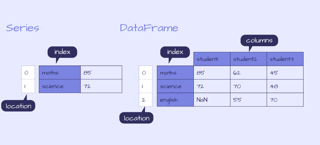Example of a pandas Series and DataFrame

3. Input and output data

Input

DataFrames can be created in a variety of ways:

A) Create an empty DataFrame: df = pd.DataFrame()

B) Input data: df = pd.DataFrame(data = data), where the input data can be in many different formats, making building a DataFrame flexible and convenient as the data you work with may be in any number of structures including a dictionary of Series and as represented in the diagram above and can be built with the following code:

d = {'student1': pd.Series([85., 72.], index=['maths', 'science']),
   'student2': pd.Series([62., 70., 55.], index=['maths', 'science', 'english']),
   'student3': pd.Series([45., 48., 70.], index=['maths', 'science', 'english'])}
df = pd.DataFrame(d)
print(df.head())

C) Input from a file or data source which we will focus on here looking at the raw CSV of the Palmer Penguin data.

Much like when building a DataFrame using input data, when creating a DataFrame from a file or data source, many input formats are accepted.

This includes:

• excel spreadsheets

• SQL

• CSV

• JSON

Check out the pandas documentation for the full list.

This offers a lot of flexibility in data storage and you can read in files that are stored locally, remotely and it even accepts compressed files.

The Palmer Penguin file we are interested is hosted on GitHub, you can download this file and read the CSV specifying the location on your machine, or we can provide the link to the raw file and open it with one line of code:

df = pd.read_csv('https://raw.githubusercontent.com/allisonhorst/palmerpenguins/1a19e36ba583887a4630b1f821e3a53d5a4ffb76/data-raw/penguins_raw.csv')

Another common data source is an SQL database. There are many different python packages to connect to the database, one example is pymysql where we can first connect to a MySQL database and then use read_sql to load the data from the query into df. This offers the flexibility to connect to remote databases quickly and easily!

Note: This is just an example of how to read in SQL data and is not used in the tutorial

# Example code: how to use read_sql
import pymysql

con = pymysql.connect(host='localhost', user='test', password='', db='palmerpenguins')

df = read_sql(f'''SELECT * FROM penguins''', con)

💡 Python 3’s f-strings are convenient to use when inputting queries.

We might later input a condition that uses a variable we have previously defined and instead of hard-coding the condition we can include the variable directly in the f-string.

The triple quotation also allows single quotes to be used within the f-string without an escape character as in the example below. For example:

# Example code: f-string's and variables
region = tuple('Anvers')

df = read_sql(f'''SELECT * FROM penguins WHERE Region IN {region} AND Date Egg > '2007-11-11' ''', con)

Large DataFrames

When reading in large datasets, it is possible to iterate over the file and read in a limited number of rows per iteration by specifying the option of chunksize to read_csv , read_sql or other input functions. However, it is worth noting that this function now returns a TextFileReader instead of a DataFrame and requires a further step to concatenate the chunks into one DataFrame.

df = read_csv('https://raw.githubusercontent.com/allisonhorst/palmerpenguins/1a19e36ba583887a4630b1f821e3a53d5a4ffb76/data-raw/penguins_raw.csv', chunksize = 10000)

df_list = []
for df in df:
    df_list.append(df)

df = pd.concat(df_list,sort=False)

This step is not necessary to use on the Palmer Penguin dataset as it’s only a few hundred rows, but is shown here to demonstrate how you could use this on a large file to read the data in 10k rows at a time.

Output

Just as we can input the file in many formats, to output a DataFrame to a file is just as flexible and easy!

After some manipulation, we can write our DataFrame to a CSV with the option to compress the file if required:

df.to_csv('output.csv', compression='gzip)

If your data is stored within AWS, there is an AWS SDK for Python, boto3 that can be used to connect to your AWS services.

4. Quick checks to inspect the data

Before we start exploring our data, the first thing to check that it has loaded correctly and contains what we expect.

Dimensions of DataFrame

We can first check that the DataFrame is not empty by checking that the number of rows is greater than 0 and further check the dimensions with the following functions:

• Get the number of rows: len(df)

• Get the number of columns: len(df.columns)

• Get the number of rows and columns: df.shape

• Get the number of elements (rows X columns): df.size

We can check this with:

if len(df) > 0:
    print(f'Length of df {len(df)}, number of columns {len(df.columns)}, dimensions {df.shape}, number of elements {df.size}')
else:
    print(f'Problem loading df, df is empty.')

This returns:

Length of df 344, number of columns 17, dimensions (344, 17), number of elements 5848

Our dataset has loaded correctly and has 344 rows and 17 columns. What does this DataFrame contain?

dtypes and memory

We’ve loaded in the DataFrame but we still don’t know what type of data it contains. We can get a summary with df.info()- let’s take a look at what details it returns:

df.info()

<class 'pandas.core.frame.DataFrame'>
RangeIndex: 344 entries, 0 to 343
Data columns (total 17 columns):
studyName              344 non-null object
Sample Number          344 non-null int64
Species                344 non-null object 
Region                 344 non-null object 
Island                 344 non-null object 
Stage                  344 non-null object 
Individual ID          344 non-null object 
Clutch Completion      344 non-null object 
Date Egg               344 non-null object 
Culmen Length (mm)     342 non-null float64 
Culmen Depth (mm)      342 non-null float64 
Flipper Length (mm)    342 non-null float64 
Body Mass (g)          342 non-null float64 
Sex                    334 non-null object 
Delta 15 N (o/oo)      330 non-null float64 
Delta 13 C (o/oo)      331 non-null float64 
Comments               54 non-null object 
dtypes: float64(6), int64(1), object(10) memory usage: 45.8+ K 

df.info() returns:

• the index data type (dtype) and range, in this case, a pandas DataFrame with 344 entries denoted by index values 0–343,

• the name and dtypes of each column, and the number of non-null values,

• the memory usage

The penguin data contains columns with mixed or string datatypes objects, integers int64 and floats float64. The table below summarises dtypes in pandas.

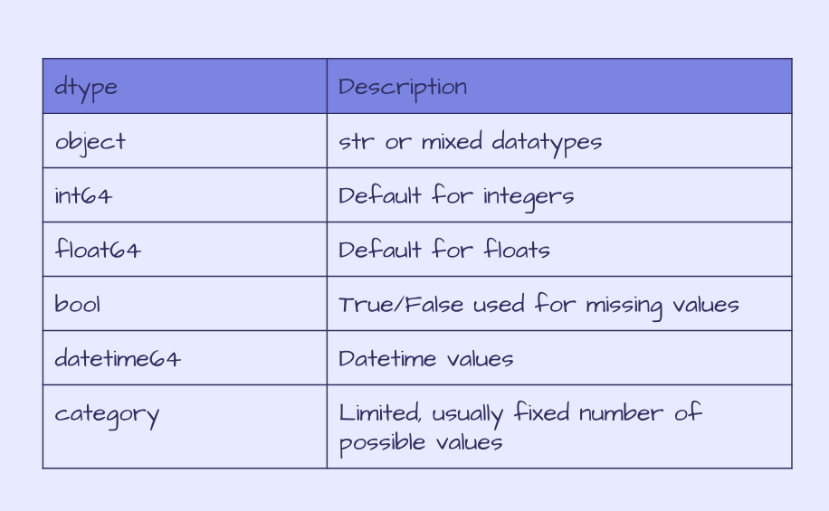Pandas dtypes

Using df.info() the memory usage by default only gives us an estimation based on the column dtype and number of rows.

We can specify to use deep introspection to calculate the real memory usage which can be particularly useful when dealing with large dataframes:

df.info(memory_usage='deep')


<class 'pandas.core.frame.DataFrame'> 
RangeIndex: 344 entries, 0 to 343 
Data columns (total 17 columns): 
studyName              344 non-null object 
Sample Number          344 non-null int64 
Species                344 non-null object 
Region                 344 non-null object 
Island                 344 non-null object 
Stage                  344 non-null object 
Individual ID          344 non-null object 
Clutch Completion      344 non-null object 
Date Egg               344 non-null object 
Culmen Length (mm)     342 non-null float64 
Culmen Depth (mm)      342 non-null float64 
Flipper Length (mm)    342 non-null float64 
Body Mass (g)          342 non-null float64 
Sex                    334 non-null object 
Delta 15 N (o/oo)      330 non-null float64 
Delta 13 C (o/oo)      331 non-null float64 
Comments               54 non-null object 
dtypes: float64(6), int64(1), object(10) memory usage: 236.9 KB

We can also check the memory usage per column with:

print(df.memory_usage(deep=True))
Index                     80 
studyName              22016 
Sample Number           2752 
Species                31808 
Region                 21672 
Island                 21704 
Stage                  25800 
Individual ID          21294 
Clutch Completion      20604 
Date Egg               23048 
Culmen Length (mm)      2752 
Culmen Depth (mm)       2752 
Flipper Length (mm)     2752 
Body Mass (g)           2752 
Sex                    21021 
Delta 15 N (o/oo)       2752 
Delta 13 C (o/oo)       2752 
Comments               14311 
dtype: int64 

Or the total memory usage with the following:

print(df.memory_usage(deep=True).sum())

242622

We can see here that the numerical columns are significantly smaller than the columns containing objects. Not only that but we aren’t interested in all the columns in our analysis.

This raw file contains all the data that has been collected. If we are to compare the body mass, flipper lengths and culmen dimensions in the different species of penguins and on the different islands, then we can clean the data and keep only the data that is relevant.

5. Data cleaning

To clean the data there are several steps we can take:

Remove columns we aren’t interested in

Let’s take a first glance at the first few rows of data:

print(df.head())

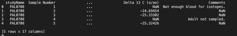Output of df.head()

This output doesn’t look quite right. We know that there are 17 columns but we can only see 4 of them plus the index here. Depending on the size of the console you are working in, you might see a few more columns here but probably not all 17.

To view all the columns, we can set the value for display.max_columns to be None.

pd.set_option('display.max_columns', None)
print(df.head())

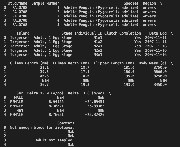Output of df.head() after setting the max columns to be None

Looking at a sample of the data, we can identify the columns that we want to use and reassigning a new value to df by specifying only the rows and columns we want to keep. We can use df.loc(rows, cols) to do this. In the rows argument, a colon denotes all values and the columns we can specify the columns we are interested in, which are: Species, Region, Island, Culmen Length (mm), Culmen Depth (mm), Flipper Length (mm), Body Mass (g), Sex

keep_cols = ['Species', 'Region', 'Island', 'Culmen Length (mm)', 'Culmen Depth (mm)', 'Flipper Length (mm)', 'Body Mass (g)', 'Sex']

df = df.loc[:, keep_cols]  

print(df.columns)  

>>> Index(['Species', 'Region', 'Island', 'Culmen Length (mm)',        'Culmen Depth (mm)', 'Flipper Length (mm)', 'Body Mass (g)', 'Sex'],       dtype='object'

We now only have the columns of interest stored in our DataFrame.

Replace or drop null values

We can check again the memory usage of df and we can see it has halved by removing irrelevant columns.

df.info(memory_usage='deep')

<class 'pandas.core.frame.DataFrame'> 
RangeIndex: 344 entries, 0 to 343 
Data columns (total 8 columns): 
Species                344 non-null object 
Region                 344 non-null object 
Island                 344 non-null object 
Culmen Length (mm)     342 non-null float64 
Culmen Depth (mm)      342 non-null float64 
Flipper Length (mm)    342 non-null float64 
Body Mass (g)          342 non-null float64 
Sex                    334 non-null object 
dtypes: float64(4), object(4) memory usage: 104.8 KB 

Looking at the number of non-null values, the size data has 2 null values and the sex has 10. We can also see this with:

print(df.isna().sum())  
Species                 0 
Region                  0 
Island                  0 
Culmen Length (mm)      2 
Culmen Depth (mm)       2 
Flipper Length (mm)     2 
Body Mass (g)           2 
Sex                    10 
dtype: int64

We can either drop these values or replace them with another value, specifying inplace=True in the function to reassign the value. In this case, we can replace the na values with Unknown for the Sex columns and we can drop the na values for the other columns.

df['Sex'].fillna('Unknown', inplace=True) 

print(df.isna().sum())  

Species                0 
Region                 0 
Island                 0 
Culmen Length (mm)     2 
Culmen Depth (mm)      2 
Flipper Length (mm)    2 
Body Mass (g)          2 
Sex                    0 
dtype: int64  

df.dropna(inplace=True) 

print(df.isna().sum())  

Species                0 
Region                 0 
Island                 0 
Culmen Length (mm)     0 
Culmen Depth (mm)      0 
Flipper Length (mm)    0 
Body Mass (g)          0 
Sex                    0 
dtype: int64

Since there were only a few values we removed, this is unlikely to impact the memory usage but is useful to clean the data and when dealing with large DataFrames with a significant number of null values, it may reduce memory.

Convert objects to Categorical dtypes

The final step in cleaning our data is to check the number of unique values in each column to determine whether a categorical dtype is more suitable in place of using objects.

We already know that there are three penguin species in our data yet the dtype for this column is an object, so let’s check this column first.

print(df['Species'].head())  

0    Adelie Penguin (Pygoscelis adeliae) 
1    Adelie Penguin (Pygoscelis adeliae) 
2    Adelie Penguin (Pygoscelis adeliae) 
4    Adelie Penguin (Pygoscelis adeliae) 
5    Adelie Penguin (Pygoscelis adeliae) 
Name: Species, dtype: object  

print(df['Species'].nunique())  

3  

print(df['Species'].unique())  

['Adelie Penguin (Pygoscelis adeliae)' 'Gentoo penguin (Pygoscelis papua)'  'Chinstrap penguin (Pygoscelis antarctica)']

As expected there are only 3 unique values in this column but each row contains a string with the penguin species, taking up significant memory. We can instead convert this column to be a category dtype and check how this changes the memory.

print(df.memory_usage(deep=True))

Index                   2736
Species                31626
Region                 21546
Island                 21575
Culmen Length (mm)      2736
Culmen Depth (mm)       2736
Flipper Length (mm)     2736
Body Mass (g)           2736
Sex                    21213
dtype: int64

df['Species'] = df['Species'].astype('category')

print(df.memory_usage(deep=True))

Index                   2736
Species                  702
Region                 21546
Island                 21575
Culmen Length (mm)      2736
Culmen Depth (mm)       2736
Flipper Length (mm)     2736
Body Mass (g)           2736
Sex                    21213
dtype: int64

This has now gone from 31626 bytes to 702, reducing the size significantly! The same approach can be taken for the other object columns, Region, Island and Sex.

for col in ['Region','Island','Sex']:
    print(f'Column: {col}, number of unique values, {df[col].nunique()}, unique values: {df[col].unique()}')

Column: Region, number of unique values, 1, unique values: ['Anvers']
Column: Island, number of unique values, 3, unique values: ['Torgersen' 'Biscoe' 'Dream']
Column: Sex, number of unique values, 4, unique values: ['MALE' 'FEMALE' 'Unknown' '.']

Region has only one value, this column can be removed since it doesn’t provide any value.

df.drop(columns=['Region'], inplace=True)
print(df.columns)

Index(['Species', 'Island', 'Culmen Length (mm)', 'Culmen Depth (mm)',
       'Flipper Length (mm)', 'Body Mass (g)', 'Sex'],
      dtype='object')

Island and Sex can be converted to categorical dtypes in the same way as Species. Before we do that, there is a strange value in the Sex column of a full-stop, let’s take a look at how many of these there are.

print((df['Sex']=='.').value_counts())

False    341
True       1
Name: Sex, dtype: int64

Since there is only 1 value, let’s replace it with Unknown in the same way that we replaced the null values.

df['Sex'].replace('.','Unknown', inplace=True)
print((df['Sex']=='.').value_counts())

False    342
Name: Sex, dtype: int64

Now we are happy with the columns, let’s convert Sex and Island to categories and check the final memory usage:

df['Sex'] = df['Sex'].astype('category')
df['Island'] = df['Island'].astype('category')

print(df.memory_usage(deep=True))

Index                  2736
Species                 702
Island                  613
Culmen Length (mm)     2736
Culmen Depth (mm)      2736
Flipper Length (mm)    2736
Body Mass (g)          2736
Sex                     610
dtype: int64

print(df.memory_usage(deep=True).sum())

15605

The total memory usage has gone from 242622 to 15605.

df.info(memory_usage='deep')

<class 'pandas.core.frame.DataFrame'>
Int64Index: 342 entries, 0 to 343
Data columns (total 7 columns):
Species                342 non-null category
Island                 342 non-null category
Culmen Length (mm)     342 non-null float64
Culmen Depth (mm)      342 non-null float64
Flipper Length (mm)    342 non-null float64
Body Mass (g)          342 non-null float64
Sex                    342 non-null category
dtypes: category(3), float64(4)
memory usage: 15.2 KB

Reducing the memory from 236.9 KB to 15.2 KB.

Mission accomplished!

We’ve so far covered how to get started with reading a file into pandas and cleaning the file to optimise performance. The penguin data is already well structured, with only minimal cleaning needed compared to the types of data you might come across from other sources. It is also a fairly small dataset starting at 200 KB when pandas can deal with files in the order of GBs, where these quick tips can yield significant improvements in performance.

This is part 1 of a series of tutorials. In the following parts, we will explore our data quantitively and graphically, creating data visualisations using pandas, and some additional python packages — matplotlib and seaborn and we will dive into some other features of pandas that are useful to know!

The full code from this tutorial can be found on GitHub!

Are there any pandas functions for data inspection and cleaning that you’d like to hear more about? Or any I’ve missed? Let me know!

If you enjoyed this article, you can subscribe to my monthly newsletter to get my latest articles, resources I use and other tips directly in your inbox!

This article is also on Medium.